
GEM Dayside Kinetics Challenge
Introduction
The GEM Focus Group Dayside Kinetic Processes in Global Solar Wind-Magnetosphere Interaction, co-chaired by Heli Hietala, Xochitl Blanco-Cano, Gabor Toth, Andrew Dimmock, is sponsoring a Dayside Kinetic Challenge [PDF]
We start this focus group on "Dayside Kinetics" with a modeling challenge where we analyze the various dayside phenomena (magnetic reconnection, FTEs, magnetosheath waves, etc.) during a short interval of steady solar wind input conditions from the first MMS dayside season. We aim to conduct comparisons between (i) observations and (global) models with different levels of kinetic physics; (ii) different models; (iii) in situ and remote observations.
The southward IMF event on 2015-11-18 01:50-03:00 UT, featuring an MMS-Geotail magnetopause conjunction with SuperDARN radar observations is set as the first challenge event.
Naritoshi Kitamura presented the event at the 2016 Summer Workshop. See a summary of the observations.
Modeling input parameters and files
Time interval, solar wind conditions (GSM) and dipole tilt. Pure proton-electron plasma is assumed (no alpha particles).
| Time | |B| | Bx | By | Bz | Vx | Vy | Vz | N | Ti | Te | dipole tilt |
|---|---|---|---|---|---|---|---|---|---|---|---|
| (UT) | (nT) | (nT) | (nT) | (nT) | (km/s) | (km/s) | (km/s) | (/cm3) | (eV) | (eV) | (deg.) |
| 01:50-03:00 | 6 | 0 | 0 | -6 | -365 | 0 | 0 | 9.5 | 9 | 9 | -27* |
*Dipole axis is tilted from the positive Z-axis towards the negative X-axis (pole in northern hemisphere is pointing away from the Sun).
Orbit information for Geotail and MMS (Re, GSM, ascii):
Target outputs and metrics
- Location of the magnetopause (based on MMS and Geotail crossings)
- Location of the X-line
(northward of the spacecraft, estimated to be at ZGSM~ 2 RE) - Thickness of the current sheet at MMS
- Properties of the FTEs (including their periodicity)
- MMS local observations
- Ground-based observations (e.g., estimated speed)
- magnetosheath magnetic field power spectrum
- properties of the magnetosheath mirror mode waves
How to participate in the challenge
Please write an email to Lutz Rastaetter and CC Heli Hietala and Gabor Toth, with your name, institution, the name of the code to be used, a brief description of the code or some reference, expected time line for producing results, which results/metrics are targeted, and whether you are interested to be a co-author in a future joint paper.
Observations
Solar Wind Conditions
Provided by: Rishi Mistry (Imperial College) and Heli Hietala (UCLA).
- Summary of the solar wind analysis:
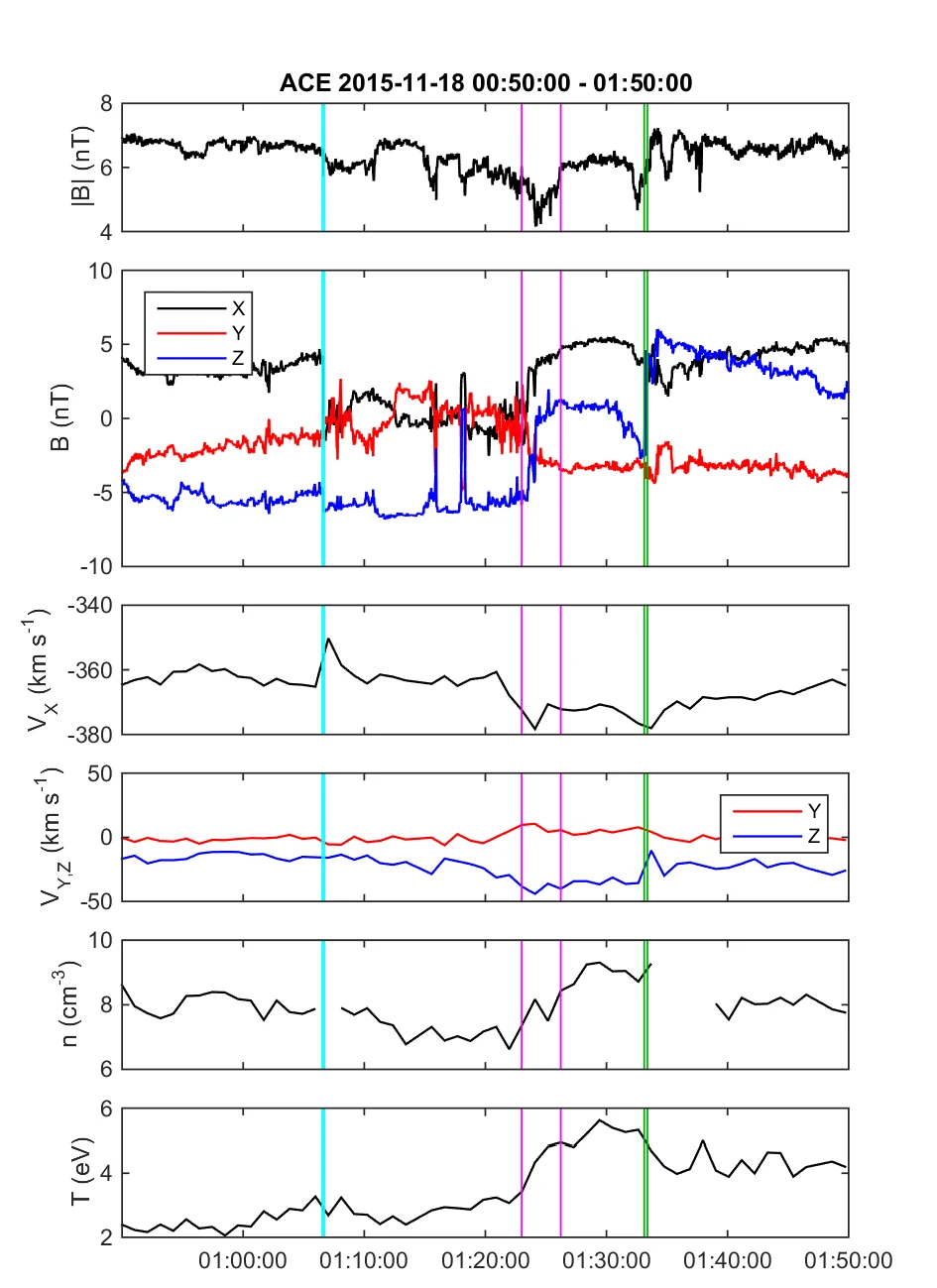
The interval of interest starts with IMF discontinuity S1 and ends with IMF discontinuity S2. The average solar wind conditions (GSM) from the solar wind analysis Excel file are:| | |B| (nT) | Bx (nT) | By (nT) | Bz (nT) | Vx (km/s) | Vy (km/s) | Vz (km/s) | n (/cm3) | Ti (eV) | Te (eV) | alpha fraction || before S1 | 6.4 | 2.7 | -2.5 | -5.1 | -360.1 | 5.0 | -2.2 | 8.2 | 8.2 | 10.3 | 0.03-0.05 || S1-S2 | 6.2 | 0.1 | -0.6 | -5.7 | -361.3 | 3.7 | -11.1 | 8.3 | 7.4 | 10.3 | 0.05-0.08 || simulate | 6 | 0 | 0 | -6 | -365 | 0 | 0 | 9.5 | 9 | 9 | 0 |Timing: Discontinuity S2 behaves consistently at all four spacecraft, and its expected arrival time at subsolar bow shock is around 2:45 UT (between 2:39 UT and 3:04 UT). This is consistent with the smooth rotation seen by MMS in the magnetosheath between 2:50 UT and 3:05 UT.Discontinuity S1, however, gives very different normal vectors at different spacecraft (it may have been non-planar), and hence wildly different arrival times: perhaps around 2:29 UT, but the spread is from 1:11 UT to 3:10 UT. In MMS magnetosheath data (about 2:15 UT ->) there is no clear evidence for a sharp rotation. The conclusion is that eitherTherefore it is possible that the IMF orientation during (some of) the MMS reconnection observations between 1:50 and 2:35 UT may have been a bit different from purely southward (see the above table), but that is uncertain and the effect is probably relatively small. . a) S1 arrived earlier, and/or . b) crossing the bow shock, S1 turned into such a smooth/weak change in the field direction that it is not clear in the MMS near-magnetopause data. - Detailed analysis of the solar wind conditions [Excel file].
Excel work sheets have solar wind conditions, bow shock arrival times for each solar wind monitor (ACE, Wind, ARTEMIS P1 and P2) and discontinuity normals. - Density and composition: . ACE SWEPAM gives alpha to proton ratio of ~0.05 between S1 and S2, and ~0.03 before S1. . Wind SWE gives alpha number density of ~0.6/cc between S1 and S2, and ~0.4/cc before S1. These correspond to ratios of 0.08 and 0.05. . Wind 3DP (on-board moments) gives alpha number density of ~0.45/cc between S1 and S2, and ~0.25/cc before S1. These correspond to ratios of 0.06 and 0.03. . In summary: before S1 there was 3-5% of alphas, and between S1 and S2 there was 5-8% of alphas. . Simulation approach: Assume pure proton plasma and use n=9.5/cc instead of 8/cc because that better represents the mass density, which actually determines the ram pressure and the magnetopause location. If n_total = 8.3/cc and 5% is alpha particles, then the mass density is 8.3*(0.95 + 4*0.05) amu/cc = 9.54 amu/cc.
- Plots of solar wind conditions from ACE, Wind, and the two ARTEMIS spacecraft (GSE)
Magnetospheric Conditions
- Further analysis results to be included. See the Dayside Kinetic Challenge [PDF] for information on the observational analysis team.
Simulation Results
- No results are available yet.