PlotMode Documentation
About
The main category of in the CCMC visualization is called PlotMode. Data can be displayed in different ways such as scalar mountain, contours or vector arrows, and multiple physical quantities can be displayed in a layered plot. Here are the PlotModes:
- Surface: The data in the 2D slice (quantity Q1 at X=constant, Y=constant, or Z=constant, see below in the select cut plane section of the form) is displayed as a mountain-like surface (Fig 1).
In the choose plot area section of the form the user can restrict the area plotted (this applies to all Plot Modes).
EarthView replaces Surface in the ionosphere visualization interface. EarthView displays the variable wrapped onto the Earth showing the continents as geographical reference. The parameters AX and AZ can be used to look at the result from different directions. - Line Plot: Up to three variables (Q1,Q2,Q3, purged of duplicates) can be plotted along any straight line through the 3-D (2-D) domain. The start point [X1,Y1,Z1] and the end point [X2,Y2,Z2] are selected in the choose plot area section of the form. Masked areas will be shown as empty space between vertical thick lines. Small tick marks on the X-axis show location of grid points.
- Vertical Plot: Data are plotted like Line Plot, but along the vertical line defined by the start point coordinates and over the entire range in the vertical (Z, H, or Alt) coordinate (Fig. 3). The data are either interpolated (101 elements) or sampled with maximum resolution (defined by the unique grid positions in the vertical direction). The vertical axis is the altitude and model output variables are plotted in horizontal direction.
- Contour: the slice is shown as a 2D plot with contours (lines with constant levels of quantity Q1).
- Vector: The components of a vector (e. g. V, B, J) in the slice plane are shown as arrows (centered on sample positions like compass needles). It is recommended to interpolate data onto an equidistant grid to get an even distribution of arrows in the plot domain.
Choose Q1 to be any component of a vector (e. g. V_x, B_z, J_y), otherwise the (scalar) choice (e. g. N or P) will be displayed as a Surface. - ColorContour: Contour plot using color-filled levels (Fig. 4). The model grid and boundaries of interest (e.g., Fok model boundary, geosynchronous orbit) can be displayed on the plot.
- Color+Vector: Combination of ColorContour plot with Vector (arrows) on top (Q1: any choice for color contour, Q2: any component of a vector, Fig. 5).
- Contour+Vector: Combination of plain Contour with Vector (Q1: any choice, Q2: component of a vector).
- Color+Contour: Combination of ColorContour and plain Contour (Q1 and Q3 are used and can be any choice of quantity).
- Color,Vector+Contour: Combination of ColorContour, Vector and plain Contour plots. This option uses all three choices Q1, Q2, Q3 for ColorContour, Vector and Contour, respectively)
- Color,Vector+Flow Lines: Combination of ColorContour,Vector and the display of vector flow lines (Q2 and Q3 must be components of a vector quantity). Fig. 6
Flow lines are traced in 3D from cut plane, but are projected onto the cut plane, available start points are pre-defined in the cut plane, random (Flow Line Setup below) and user-defined. - 3D-Flowlines: This plot (Fig. 6) option uses variable Q1 to generate
- magnetic field lines for B, or B1 (adding analytical expression for dipole if B1 is selected),
or - flow lines for V, J, E, etc..
Field lines and flow lines are traced in 3D, starting from predefined starting points and user-defined starting points according to the selection of the Flowline Setup Mode that determines the distribution of pre-defined start points.
- Color Contour on Sphere: Using the radius of the exclusion area it is possible to render a sphere with the scalar quantity Q1 in color (Fig. 9). Interpolated values at the positions used for the plot can also be written to ASCII text files returned to the user. The view direction is controlled by the view angles AX (elevation angle in degrees) and AZ (azimuth angle from negative Y-axis).
- SWX 3D-Flowlines: This plot (Fig. 8) option uses variable Q1 to generate
- magnetic field lines for B, or B1 (adding analytical expression for dipole if B1 is selected),
or - flow lines for V, J, E, etc..
Field lines and flow lines are traced in 3D, starting from predefined starting points and user-defined starting points according to the selection of the Flowline Setup Mode that determines the distribution of pre-defined start points.
- SWX Slice:(Fig. 10) Creates a slice through the 3D data, with the variable Q1 mapped to color.
- SWX Flowlines + Contour Slice:(Fig. 13) Uses variable Q1 to generate flowlines and variable Q2 to generate the slice.
- SWX Slice-SurfacePlot:(Fig. 14) A surface plot version of the slice visualization. See the surface plot description above. Uses variable Q1 to generate the slice.
- SWX Contour Slice-SurfacePlot:(Fig. 15) A surface plot version of the contour slice visualization. See the surface plot description above. Uses variable Q1 to generate the slice.
- SWX Flowlines+Slice-SurfacePlot:(Fig. 16) Uses variable Q1 to generate flowlines and variable Q2 to generate the slice.
- SWX Flowlines+Contour Slice-SurfacePlot:(Fig. 17) Uses variable Q1 to generate flowlines and variable Q2 to generate the slice. |
General Options For All PlotModes
Note: "X", "Y", "Z" stand here not only for the Cartesian coordinates but also for the names of the first, second, and third coordinates of any model grid (e. g., radius "r", longitude "lon", and latitude "lat" for a spherical grid).
Selection of plot area
These fields are only present for the interface accessing three-dimensional data (see options for two-dimensional data below).
- Near the bottom of the form, the boundaries of the plot region ( start and end point of a line plot) are defined by X1,Y1,Z1, and X2,Y2,Z2.
The selection of and the location of the Cut Plane can be specified within the ranges given for X, Y and Z.
Exclude Region
A certain region around the central body (Earth, Sun, or other object, depending of model and domain) can be excluded from a plot (changing the automatically calculated plot data range).
In 2D slice plots, the excluded region shows up as a black disk around the origin with the (partially sunlit) Earth in center, if applicable.
In Line plots, no data are displayed in the excluded region which is bounded by vertical lines in the plot.
3D-Flowline plots show a ball at the origin representing the location of the Earth, the Sun or any other "Central body" future models may have). The ball radius is either the radius of the body or is specified by the radius of the excluded region.
Options for Flow lines:
Flow lines are set up with pre-defined start points in the plot area selected with field lines starting at the inner boundary or the boundary of the excluded region, along the X-axis (Earth magnetosphere), along the box boundaries (upstream boundary for velocity in global magnetosphere). Special separation lines such as the solar coronal neutral line (PFSS, at outer radius of domain).
- only user-defined start points: only computes flow lines from the list of points entered for X,Y,Z.
NOTE: User-defined points are always used with the other selections of the Flowline Setup Mode. Leave at least one of the input fields blank if no user-defined flow lines are desired. - predefined in 3D (default): evenly spaced along and parallel to the X-axis for B, 10x10 points on upstream surface (XMAX) for velocity V, 3D grid (5x5x5) in volume for other variables (J, for example)
- random in 3d -uniform: starting points are chosen randomly in X,Y,Z with uniform probability density
- random in 3d - concentrated in center of box: starting points are chosen randomly in X,Y,Z with probability density concentrated in the center of the selected view box (not at the origin!)
- predefined in cut plane: like predefined in 3D, but with 3rd coordinate projected onto the selected cut plane (X=constant, Y=constant, or Z=constant)
- uniform random in cut plane: like random in 3D - uniform, but with 3rd coordinate projected onto selected cut plane (X=constant, Y=constant, or Z=constant)
- random in cut plane - concentrated in center: like random in 3D - concentrated in center of box, but with 3rd coordinate projected onto selected cut plane (X=constant, Y=constant, or Z=constant)
Flow lines are tracked up to the inner boundary (boundary near the "Central Body") of the simulation domain.
Flow lines are color-coded depending on their connection to the inner boundary:
- Flow lines traced from pre-defined start points:**Flow lines traced from start points selected by user:**
The user can specify X,Y,Z positions of start points in three text fields in the interface. The shortest array in any of the three coordinates determines the number of start points.- blue: flow lines not connected to the Central Body (i.e., the inner boundary)
- black: flow lines are connected to the Central Body on one end ("open" or "polar Cap" field lines for B)
- red: flow lines connected to the Central Body on both ends ("closed" field lines of B)
- light blue: flow lines not connected to the Central Body, e. g., Solar wind field lines of B.
- purple: flow lines are connected to the Central Body (i.e., the inner boundary) on one end, e. g., "open", "polar Cap" or "Coronal Hole" field lines for B.
- orange: flow lines connected to the Central Body on both ends, e. g., "closed" field lines of B.
ASCII output options:
Raw data may be returned to the user by checking and selecting the following options:
- List Data Check this to get any kind of ASCII data listing.
- At Positions Specified returns the selected variables (Q1, Q2, Q3) at the specified locations. Number of data points represents number of elements in shortest array of locations.
Use combination of positions in a 3D grid: This option combines all positions for the three coordinates into a 3D grid of positions. The number of positions returned is the product of the lengths of the three arrays of coordinate positions. - List Data From Plot acts differently, depending on PlotMode selected:
- 2D plots (of any kind - Contour, Vector, Surface, combinations): data from the cut slice in the requested plot area is returned (for up to 44,000 positions on the original grid or resampled onto an equidistant 61x61 grid if Interpolate data onto equidistant grid is checked), for example:
- Line Plot: data is returned along the line plotted (either interpolated (31 elements) or with maximum resolution (defined by the largest number of unique grid positions in either coordinate between the start and end point).
- Vertical Plot: data is returned along the vertical line defined by the start point coordinates and over the entire range in the vertical (Z, H, or Alt) coordinate, either interpolated (31 elements) or with maximum resolution (defined by the unique grid positions in the vertical direction).
- 3D-Flowlines Returns for each flow line: coordinates of the start point and of each of the two end points, topology information (connectivity of flow line to 3.5 RE boundary), and exit status of the flow line tracer for both integration directions (parallel and anti-parallel to vector field). Other pieces of information may be obtained from the flow line tracings in the future.
Example: map along fieldline to ionosphere
- Prepare interface for a 3D Flowlines plot by entering user-defined start points that are interesting, e.g.,
    X: 6, 7, 8, 8, 8, 9,11
    Y: 0, 0,-3, 0, 3, 0, 0
    Z: 0, 0, 0, 0, 0, 0, 0
This establishes 7 start points.
- Check List Data and select List Data from Plot
- Make plot.
The output returned looks like this:
- X0,Y0,Z0 are the start points,
- X1,Y1,Z1 and X12,Y2,Z2 the end points of each flow line
- topo is the field line topology
- S1 and S2 the return status of the tracing of each flow line segment (tracing with and against vector orientation at start point).
    # Data printout from CCMC-simulation:
    # Data type:  BATSRUS refined V6 IDL
    # Run name:    Lewis_Franklin_082205_1
    # Date, time:         2004          12          27  22:00:00
    # Output data: GSM [R_E], flow line start and two end locations: 7 flow lines, 12, entries per line.
    # topo: 0: closed, 1: Polar Cap / open, 2: IMF / disconnected from the Earth
    # s1,s2, exit status of parallel, antiparallel trace of B1:
    #  -2: tracing not started (start point outside simulation domain or inside       3.00000 R_E)
    #   0: end inside simulation range (connected to Earth)
    #   1: end outside 3.00000 R_E (connected to IMF)
    #   2: iteration reached maximum number of steps (incomplete flow line or stalled iteration)
    #   x0      y0      z0          x1      y1      z1      x2      y2      z2       topo  s1  s2
    6.000    0.000    0.000    0.952    0.048    2.808    2.594   -0.018   -1.485  0  0  0
    7.000    0.000    0.000    0.704    0.051    2.869    2.427   -0.024   -1.687  0  0  0
    8.000   -3.000    0.000    0.299   -0.413    2.925    2.135   -0.484   -1.973  0  0  0
    8.000    0.000    0.000    0.473    0.049    2.912    2.303   -0.030   -1.882  0  0  0
    8.000    3.000    0.000    0.322    0.522    2.911    2.138    0.419   -1.978  0  0  0
    9.000    0.000    0.000    0.223    0.047    2.972    2.118   -0.037   -2.091  0  0  0
11.000 0.000 0.000 2.808 0.138 48.078 11.007 -0.093 -48.085 2 1 1- From the end points of the flow lines (in the global magnetosphere model) one can map along the magnetic dipole field to the ionosphere using utilities such as GEOPACK.
Options that modify appearance of plots:
- Exclude region around the "Central Body" ("Earth" or "Sun") has two controls:
- Checkbox to enable exclusion of area around central body (origin). Data values inside the area do not contribute to the reported data minimum and maximum in automatic (color) scale generation and for vectors.
- Text field to enter radius of exclusion region. The radius can be set to exclude, for example, the strong magnetic field near the Earth to see variations in areas farther away, such as the magnetotail current sheet or the magnetopause. Default is set to a radius suitable for this (in case of Earth magnetosphere: radius=6) or the radius of the inner boundary of the simulation region.
- Image Magnification: Default is 1.0 - the plot image size can be enlarged by factors of 1.25, 1.5 or 2 for improved image resolution, or reduced to 0.75 of the standard size (e.g., the plots in this page).
The plot interfaces now allow the download of an equivalent image in Encapsulated Postscript format suitable for presentations and publications. - Allow variable plot image size: select to get to-scale representation of lengths (within aspect ratio range (plot region width/height) of 0.3 to 4). If not selected, the plot image will be 1.8 times wider than high (630x350 pixels in default size).
- Show Grid:: Display point positions where model output data are located (cell boundaries for BATSRUS block-adaptive grid). The grid of the LFM magnetosphere model is only displayed for cut planes Y=0 Y=0 or Z=0 (LFM output data are always interpolated onto regular grid before rendering).
- latitude-MLT/LT grid: Show circles in 10° increments and 8 local time meridians on the polar plot.
- simulation grid: render positions of ionosphere grid (LFM ionosphere: grid is obtained by mapping magnetospheric grid positions closest to Earth along magnetic dipole field).
- Interpolate data onto regular grid: Display model data after interpolation onto regular grid: Default for large plot regions where number of grid points exceeds 201x201 positions. This can cause regions of fine resolution (usually near the central body) to appear ill-resolved. Sufficient reduction of the plot region will ensure that every point in the model grid is used in the plot.
Selection of interpolate data onto equidistant grid will force vector arrows to be distributed evenly throughout the plot region and not on a subset of original grid positions. - View Angles: For plots with 3D bounding box having horizontal coordinates "X" and "Y", and vertical coordinate "Z" (names of coordinates vary with plot area selected and quantity displayed):
- AX: View angle around X-axis; elevation angle of viewer position.
- AZ: View angle around Z-axis; azimuth angle of viewer position (measured clockwise from negative Y axis).
- Use Grayscale: Changes default color table (rainbow scale) to gray scale and reduces the number of color levels in contour plots from 31 to 13).
- Lock color range: select to fix color contour scale range between plots. Text fields allow to specify minimum and maximum value represented by the color range.
- Log scale: Render non-negative quantities in (base-10) logarihmic scale. Data are converted to log10 values and prefix "log" is added to the quantity name.
- Show values with contour levels: show numeric values of contour levels.
- Length of Arrows: Selection of factor larger than 1 boosts length of vector arrows that by default are scaled not to overlap with arrows centered at neighboring positions (vector arrows are "compass needles", not "vanes").
- Plot to VRML: 3D Flow Line plots can be rendered into Virtual Reality Markup Language (VRML) files. A download link will be provided when the plot images are returned.
VRML files can be viewed in web browser plug-ins such as the Cortona VRML Client.
Plot options for 2D ionosphere:
- Plot Hemispheres:
- Both: Show polar plots for both hemispheres (default).
- North: Show northern hemisphere only.
- South: Show southern hemisphere only.
Cut plane and plot area selections described for the 3D interface are replaced by the following, simpler interface options:
- Minimum latitude: Lowest latitude of polar plots.
- Choose cut meridian: Check box for meridional plot. Enter local time of cut into text box.
- Choose cut latitude: Check box for constant-latitude plot. Enter latitude of cut into text box.
List of Figures
Figure 1: Single quantity data as elevation plot

Figure 2: EarthView Plot
Earthview is available for ionospheric data plotted at constant altitude.
Figure 3: Vertical Line - Multiple quantities along line in Z
Figure 4: Color Contour (with model grid)
Single variable in color with model grid (Fok Ring Current: irregular Lagrangian grid).
Figure 5: Color Contour and Vector
Variable shown in color is named with color bar, vector variable and largest amplitude printed in upper right. Outline of continents establishes reference to geographic coordinates
Figure 6: 3D Flow Line plot
Name of variable shown at end of Z axis. Line colors as in 2D flow line plots. In this example, a series of user-selected field line start points (at 15° intervals at 3 RS) was provided in addition to the pre-defined start points on the solar surface.
Figure 7: Color Contour, Vector, and Flow Line
Name of variable in third layer (flow lines) is shown in the center of the right margin: Colors of flow lines are selected depending on their connectivity to the central body (Earth).
Figure 8: SWX 3D Flow Line plot
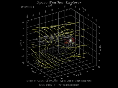
Figure 9: Color Contour on Sphere
Scalar variable rendered in color on sphere around the central body (here: Earth)

Figure 10: SWX Slice
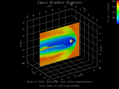
Figure 11: SWX Contour Slice
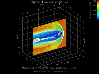
Figure 12: SWX Flowlines + Slice
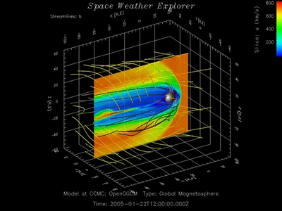
Figure 13: SWX Flowlines + Contour Slice
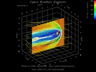
Figure 14: SWX Slice-SurfacePlot

Figure 15: SWX Contour Slice-SurfacePlot
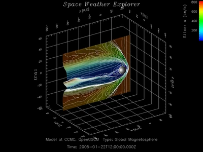
Figure 16: SWX Flowlines + Slice-SurfacePlot
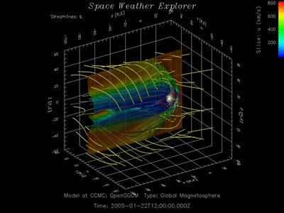
Figure 17: SWX Flowlines + Contour Slice-SurfacePlot

Figure 18