
GEM Dayside Kinetics Challenge
Go back to introduction.
Timing: Discontinuity S2 behaves consistently at all four spacecraft, and its expected arrival time at subsolar bow shock is around 2:45 UT (between 2:39 UT and 3:04 UT). This is consistent with the smooth rotation seen by MMS in the magnetosheath between 2:50 UT and 3:05 UT.
Discontinuity S1, however, gives very different normal vectors at different spacecraft (it may have been non-planar), and hence wildly different arrival times: perhaps around 2:29 UT, but the spread is from 1:11 UT to 3:10 UT. In MMS magnetosheath data (about 2:15 UT ->) there is no clear evidence for a sharp rotation. The conclusion is that either
b) crossing the bow shock, S1 turned into such a smooth/weak change in the field direction that it is not clear in the MMS near-magnetopause data.
Observations:
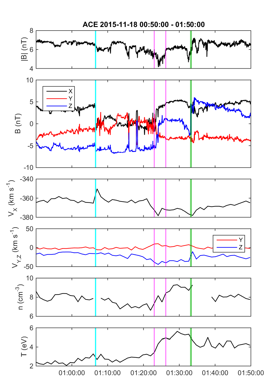
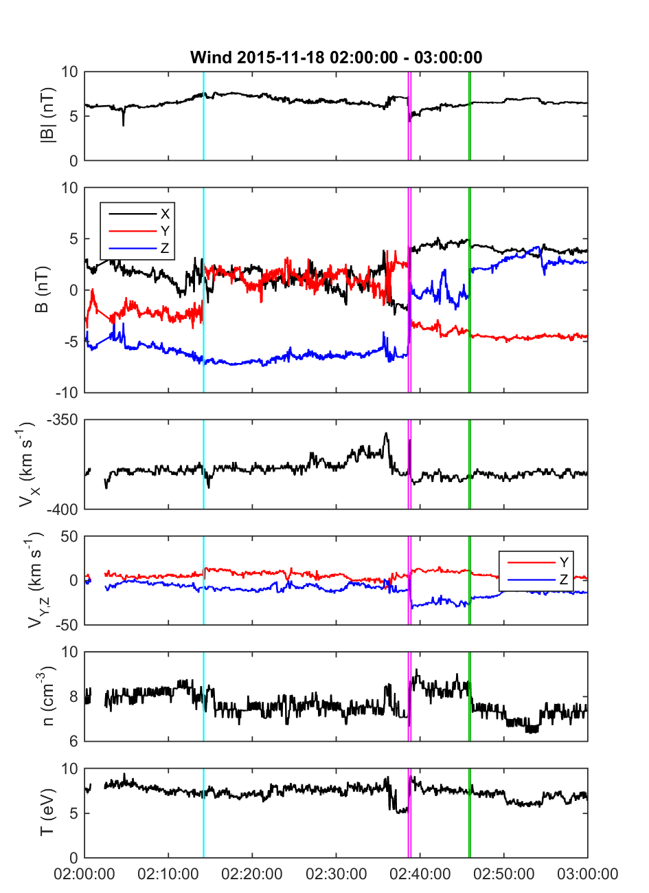
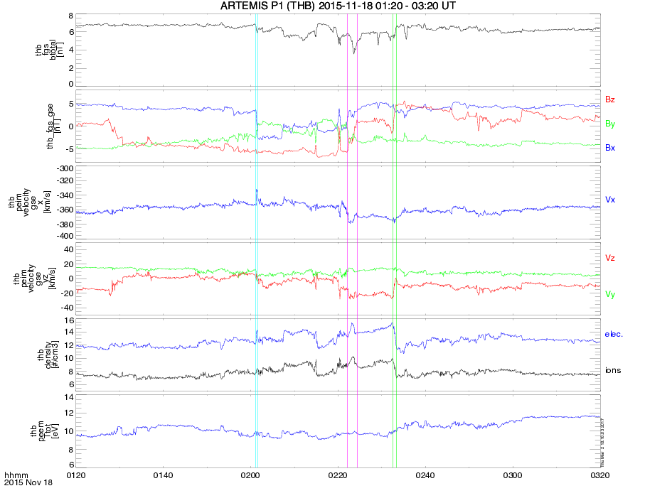
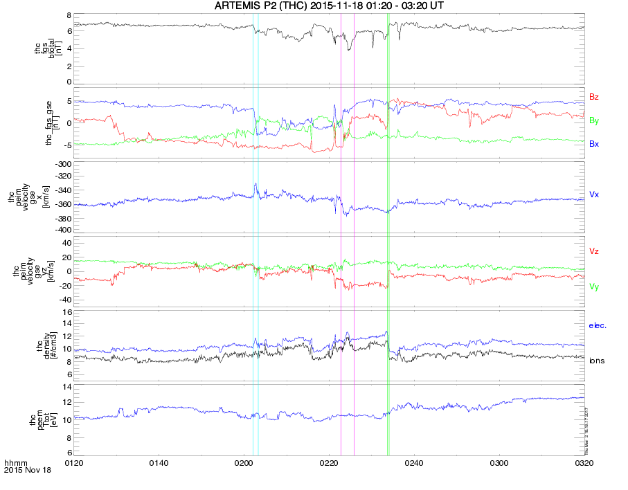
Solar Wind Conditions
Provided by: Rishi Mistry (Imperial College) and Heli Hietala (UCLA).
The interval of interest starts with IMF discontinuity S1 and ends with IMF discontinuity S2. The average solar wind conditions (GSM) from the solar wind analysis Excel file are:
|B| (nT) Bx (nT) By (nT) Bz (nT) Vx (km/s) Vy (km/s) Vz (km/s) n (/cm3) Ti (eV) Te (eV) alpha fraction before S1 6.4 2.7 -2.5 -5.1 -360.1 5.0 -2.2 8.2 8.2 10.3 0.03-0.05
S1-S2 6.2 0.1 -0.6 -5.7 -361.3 3.7 -11.1 8.3 7.4 10.3 0.05-0.08
simulate 6 0 0 -6 -365 0 0 9.5 9 9 0
a) S1 arrived earlier, and/or
Therefore it is possible that the IMF orientation during (some of) the MMS reconnection observations between 1:50 and 2:35 UT may have been a bit different from purely southward (see the above table), but that is uncertain and the effect is probably relatively small.
Excel work sheets have solar wind conditions, bow shock arrival times for each solar wind monitor (ACE, Wind, ARTEMIS P1 and P2) and discontinuity normals.
Magnetospheric conditions
Modeling results
CCMC Contact: Lutz Rastaetter
Last modified: Mar. 10, 2017