New Horizons Mission Support
"New Horizons Flyby Modeling Challenge"
Community-wide effort to provide solar wind modeling support for the New Horizons Flyby
This site presents initial results from computer simulations of the near Pluto Solar wind environment for the time period of the New Horizons Spacecraft flyby. Results are presented from models that range from a simpler 1D gasdynamic approximation, a 2D magnetohydrodynamic(MHD) simulation that includes passage of nearly 120 interplanetary coronal mass ejections, and 3D multi-fluid and 3D multiscale Fluid-Kinetic MHD models. Click on the caption in the slider for detailed results from and information about each model.
Current Contributors List
- Tae Kim
- Nikolai Pogorelov
- Gary Zank
- Dusan Odstrcil
- Bertalan Zieger
- Merav Opher
- Gabor Toth
- Tamas Gombosi
- Arcadi Usmanov
- Kenneth Hansen
- Nathan Schwadron
- Peter MacNeice (Project/Challenge Facilitator)
3D New Horizons ENLIL Simulations from the CCMC Runs-on-Request-Database
| Event Date | Run Number | Key Words | Model Type | Model | Model Version | Carrington Rotation Start | Carrington Rotation End | Start Date | End Date |
|---|---|---|---|---|---|---|---|---|---|
| Modeled Run | Leila_Mays_111215_SH_1 | New Horizons reg5med2 donkiv500w25 v3 20150201-20150431 | Heliosphere | ENLIL | 2.8 | 2159 | 2159 | 2015/02/01 00:00 | 2015/04/02 00:00 |
| Modeled Run | Leila_Mays_110815_SH_1 | New Horizons reg5med1 donkiv500w25 v3 20150201-20150431 | Heliosphere | ENLIL | 2.8 | 2159 | 2159 | 2015/02/01 00:01 | 2015/04/02 00:01 |
| Modeled Run | Leila_Mays_100215_SH_1 | New Horizons reg40low1 donkiv500w25 v1 20150201-20150901 | Heliosphere | ENLIL | 2.8 | 2159 | 2159 | 2015/02/01 00:03 | 2015/09/01 00:05 |
| Modeled Run | Leila_Mays_121215_SH_1 | New Horizons reg40low1 donkiv500w25v4 v4 20151014-20150414 | Heliosphere | ENLIL | 2.8e | 2155 | 2155 | 2014/10/14 00:04 | 2015/04/14 00:01 |
| Modeled Run | Leila_Mays_100116_SH_1 | New Horizons reg40low1 donkiv500w25v5 v5 20141014-20150414 | Heliosphere | ENLIL | 2.8f | 0 | 0 | 2014/10/14 00:00 | 2015/04/14 00:03 |
Modeling Challenge Results
1D gasdynamic model
Results from a 1D gasdynamic model of the Solar Wind propagating from the inner heliosphere to Pluto from Peter MacNeice and Nathan Schwadron.
This model solves the 1D gasdynamic equations for the Solar Wind. It includes estimates for enhancement of the wind mass density due to photoionization of neutral hydrogen entering the heliosphere from the interstellar medium. It also includes the drag effect and associated heating of the wind caused by charge exchange between protons in the solar wind and the neutral hydrogen (producing the so called Pick up ions). These source terms for these effects are implemented as in Schwadron et al (2011), Ap.J. volume 731:56. The distribution of neutral hydrogen has been set in accordance with the analysis of New Horizon SWAP measurements reported in Randol et al (2012), Ap.J. volume 755:75.
The left panels show the wind evolution as a function of radius. The vertical blue line indicates the radial location of Pluto. The right panels show the wind properties as a function of time at Pluto. The blue dot indicates the value at the time of the New Horizon flyby. This simulation is driven by the OMNI measurements of the Solar Wind in the 'near Earth' environment at 1AU. These observations have been shifted in time to account for the time varying difference in heliospheric longitude between the Sun-Earth and Sun-Pluto directions.
This second graphic shows results from the same model, but with the addition of an estimate of the additional heating due to dissipation of turbulent fluctuations in the magnetic field and solar wind velocity. These affects are modeled following the description in Adhikari et al (2014), Ap.J. volume 793:52. In this case we include the additional driving of the turbulence by the Pick Up ion population. This graphic shows results for the case in which this term is most effective, i.e. where the fraction of the pick up ion energy transferred to excited waves is largest (fd=1.0) and full mixing of incoming and outgoing waves (Γ=1.0).
The third graphic shows a similar view as the second, but in this case the timelines shown in the right hand panels record the solution at the location of the New Horizons spacecraft.
Preliminary 2D ENLIL Results from D. Odstrcil
The animations below illustrate the prediction of the solar wind parameters at the New Horizons spacecraft during its cruise phase to Pluto. Numerical simulations of more than 120 Coronal Mass Ejections (CMEs) during the past six months were performed using the heliospheric code ENLIL (Sumerian god of wind), developed by Dr. Dusan Odstrcil. ENLIL is implemented at the Community Coordinated Modeling Center (CCMC) located at NASA GSFC and utilized by NOAA Space Weather Prediction Center (SWPC) in operational space weather forecasting. Kinematic parameters of all CMEs are measured and stored in the web-accessible Database Of Notifications Knowledge Information (DONKI) by the CCMC's Space Weather Research Center (SWRC) team, while continuously monitoring space environment conditions in inner heliopshere in support of NASA's missions. Application to the outer helioshere is beyond the model's current capabilities and this simulation serves as an estimate. Solar wind would need around 4-5 months to propagate from the Sun to Pluto. All CMEs fitted by CCMC/SWRC in the last six months were used by ENLIL to estimate the disturbed solar wind parameters up to four months in the future. Although inaccuracies in the arrival times can be 2-3 weeks, this simulation estimates that Pluto might be immersed in a rarefaction region with very low solar wind densities, lasting for about one month, followed by a large merged interaction region in which a large increase of the ram pressure may significantly compress Pluto's atmosphere. In-situ measurements by New Horizons would provide important information toward sophistication and calibration of this and other heliospheric models.
Principal Investigator Dusan Odstrcil leads an effort to develop the "next-generation ENLIL code". This work is sponsored by NASA Living With A Star (LWS) program and supported by NASA/CCMC.
- Click here for an iSWA layout with interactive movies of the preliminary 2D ENLIL New Horizons simulations. Please note: accessing this link will load three 8-month simulations, please be patient while the simulations load.
2D ENLIL preliminary modeling results from 1 January 2015 to 29 August 2015 showing (a) a global view normalized solar wind number density (N R^2) contour plot in the ecliptic plane from 0.1 to 40 AU, (b) a detailed 18 AU zoom-in view at New Horizons indicated by the white box in the global view, and (c) the temporal profile of the normalized solar wind number density at New Horizons. New Horizon's trajectory is shown as white line. This simulation uses approximately 120 CMEs (with speeds > 500 km/s) within the past 8 months fitted in real-time by CCMC/SWRC, available from the DONKI database. The CME drivers are outlined in black in the (a) ecliptic plane view, and marked as the yellow periods in the (c) solar wind normalized number density profile at New Horizons. Application to the outer helioshere is beyond the model's current capabilities and this simulation serves as an illustrative concept.
2D ENLIL preliminary modeling results from 1 January 2015 to 29 August 2015 showing (center) a global view normalized solar wind number density (N R^2) contour plot in the ecliptic plane first showing the inner planet field of view from 0.1 to 2 AU, then zooming out to 40 AU. To the left and right of the contour plot are temporal profiles of the normalized solar wind number density at various NASA spacecraft throughout the solar system. New Horizon's trajectory is shown as white line. This simulation uses approximately 120 CMEs (with speeds > 500 km/s) within the past 8 months fitted in real-time by CCMC/SWRC, available from the DONKI database. The CME drivers are outlined in black in the (center) global ecliptic plane view, and marked as the yellow periods in the solar wind normalized number density profiles (left and right) at varios spacecraft. Application to the outer helioshere is beyond the model's current capabilities and this simulation serves as an illustrative concept.
2D ENLIL preliminary modeling results from 1 January 2015 to 29 August 2015 showing (center) a global view normalized solar wind number density (N R^2) contour plot in the ecliptic plane first showing the inner planet field of view from 0.1 to 2 AU, then zooming out to 40 AU, before zooming back into Pluto. To the left and right of the contour plot are temporal profiles of the normalized solar wind number density at various NASA spacecraft throughout the solar system. New Horizon's trajectory is shown as white line. This simulation uses approximately 120 CMEs (with speeds > 500 km/s) within the past 8 months fitted in real-time by CCMC/SWRC, available from the DONKI database. The CME drivers are outlined in black in the (center) global ecliptic plane view, and marked as the yellow periods in the solar wind normalized number density profiles (left and right) at varios spacecraft. Application to the outer helioshere is beyond the model's current capabilities and this simulation serves as an illustrative concept.
Concept of space weather predictions for NASA missions at the outer planets
The animations below show that a similar concept for space weather prediction with ENLIL can be applied to other NASA missions at the outer planets, such as Cassini and Juno.
Cassini
Juno
Preliminary three-fluid 3D MHD results from Arcadi Usmanov
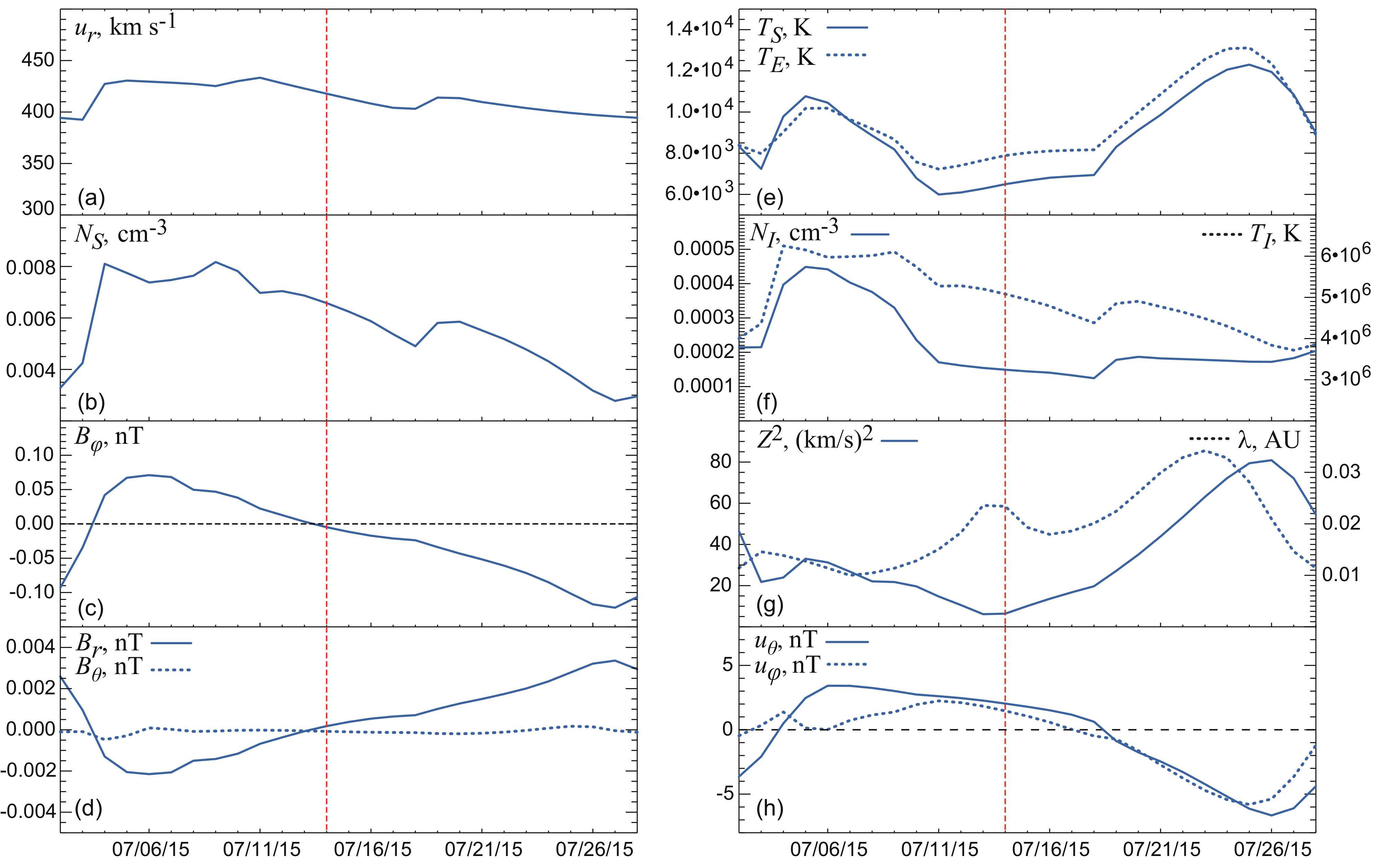
The plot below shows preliminary results from a three-fluid 3D simulation using the global solar corona and solar wind model described in Usmanov et al. (Astrophys. J., 788, 43, 2014). The output from the model is a steady-state solution in the rotating frame in the region from the coronal base to the outer heliosphere. The synoptic solar magnetogram for Carrington Rotation 2161 (February 28 - March 27, 2015) from Wilcox Solar Observatory was used for assigning boundary conditions at the coronal base. The plot shows computed variations of flow, magnetic field and turbulence parameters along the New Horizons spacecraft trajectory from July 2 to July 28, 2015 in the heliographic coordinates. The trajectory data are from OMNIWeb.
The parameters include: (a) the radial velocity ur, (b) the thermal proton density NS, (c) the azimuthal magnetic field Bφ, (d) the radial Br and meridional Bθ magnetic field components, (e) the thermal proton TS and electron TE temperatures, (f) the pickup proton density NI and pickup proton temperature TI, (g) (twice) the turbulence energy per unit mass Z2 and the correlation length of turbulence λ, and (h) the meridional uθ and azimuthal uφ velocity components. The dotted red vertical line indicates the flyby closest approach to Pluto on July 14, 2015. The computed sector boundary appears to be close to the flyby closest approach date.
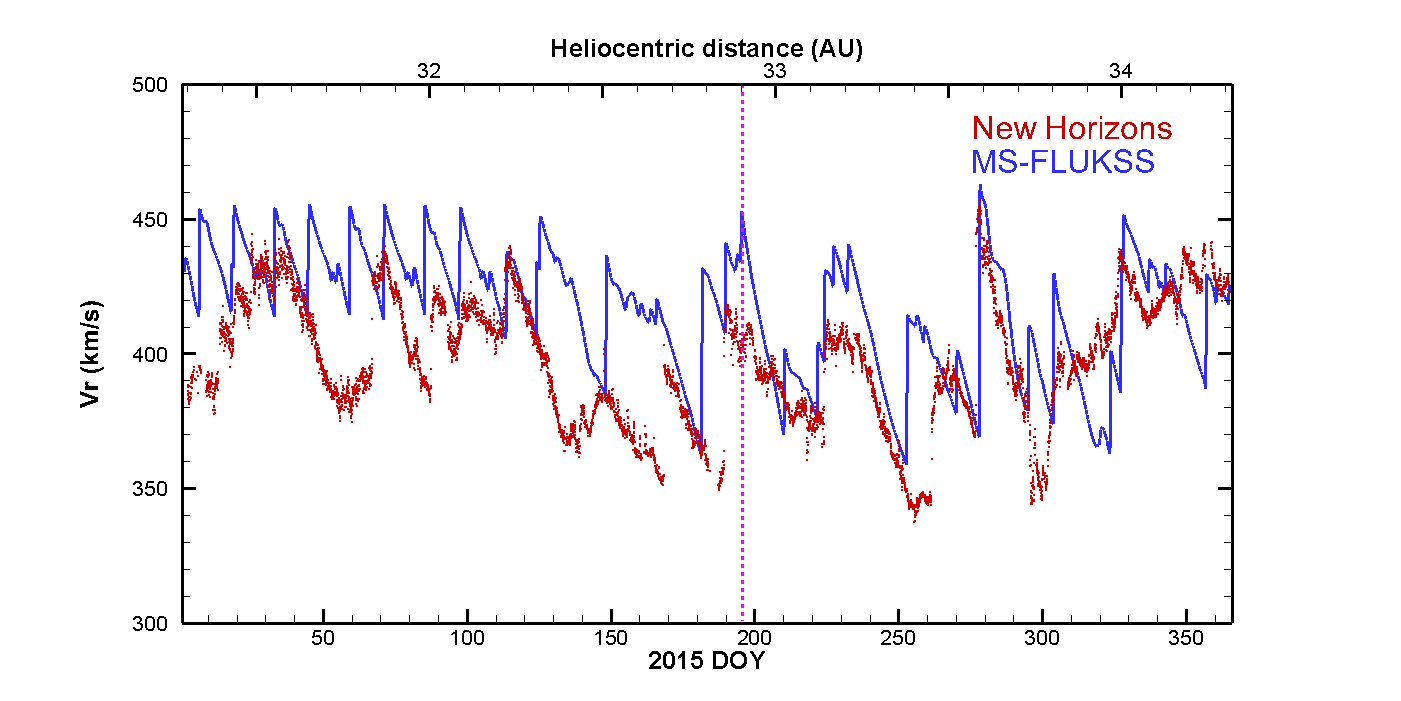
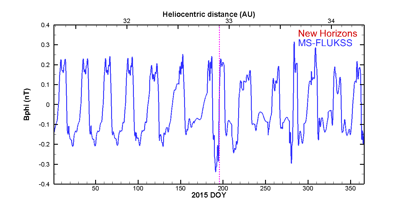
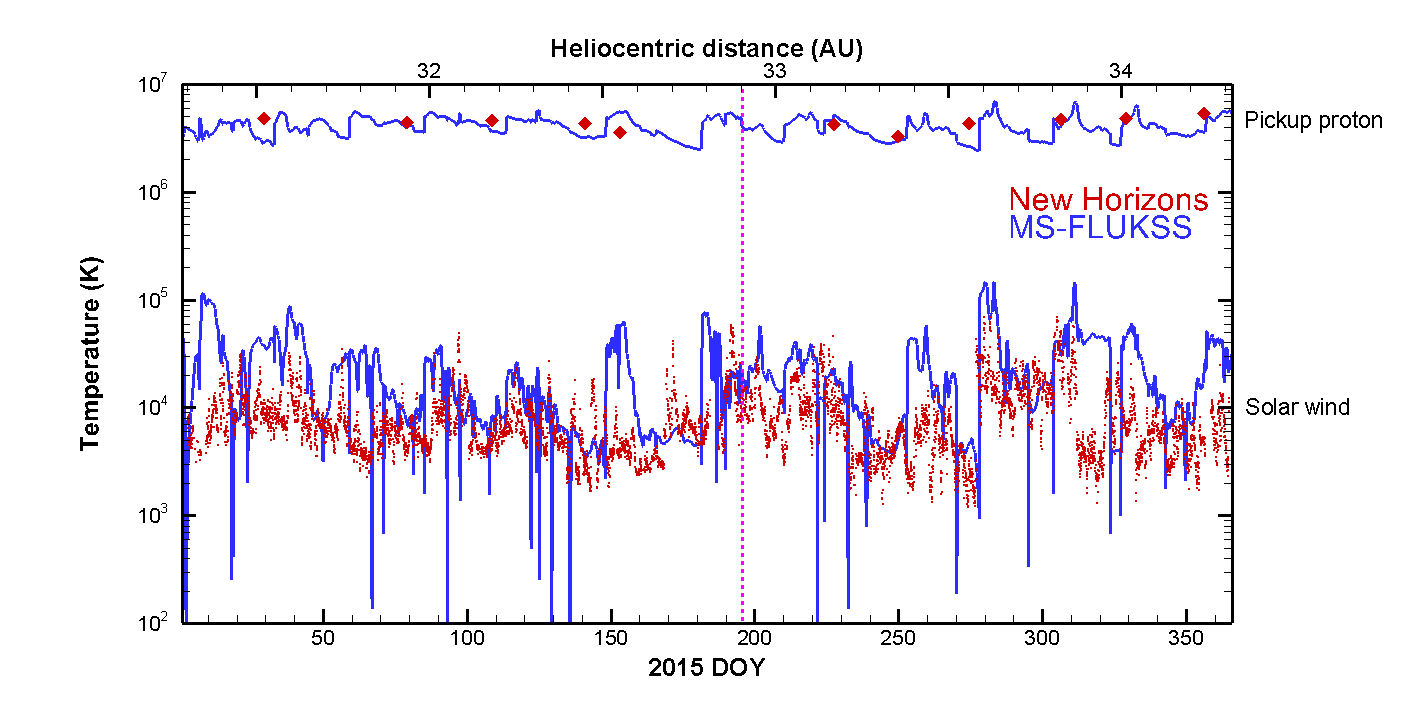
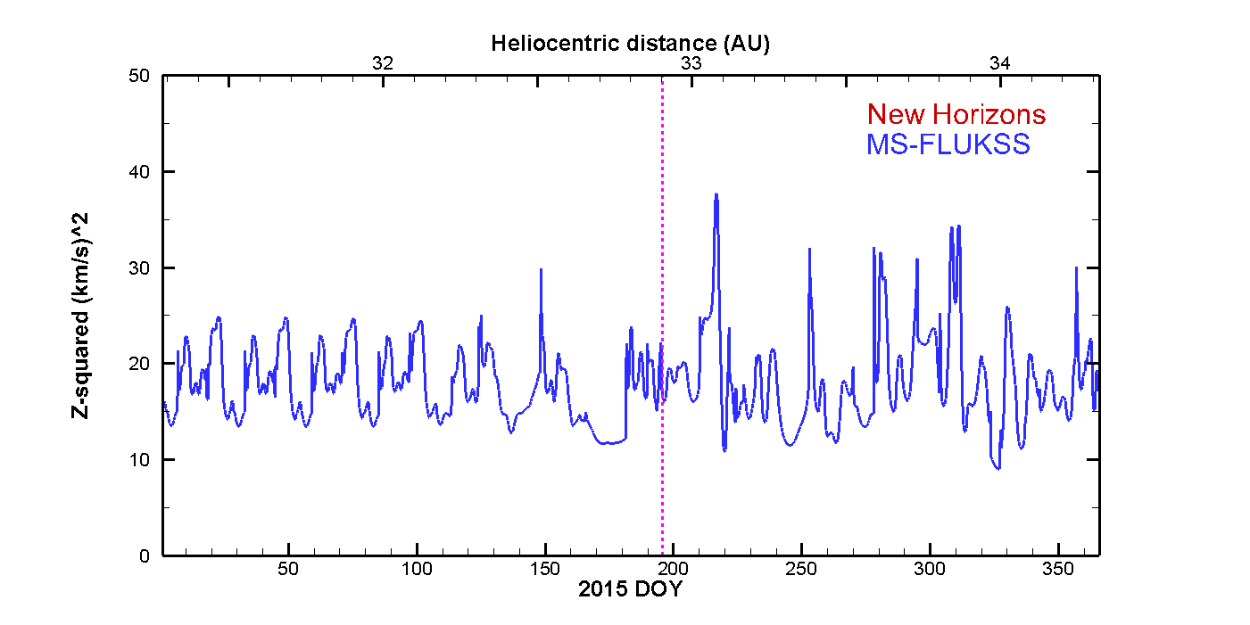
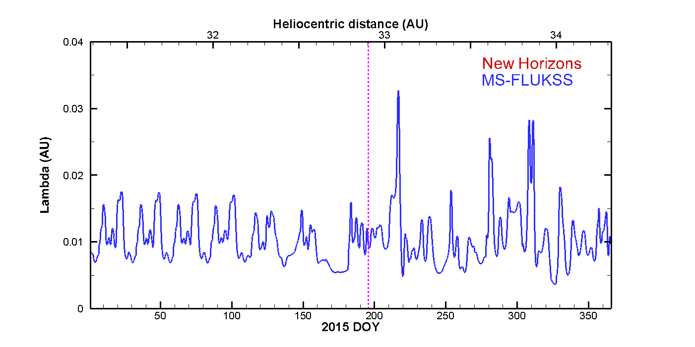
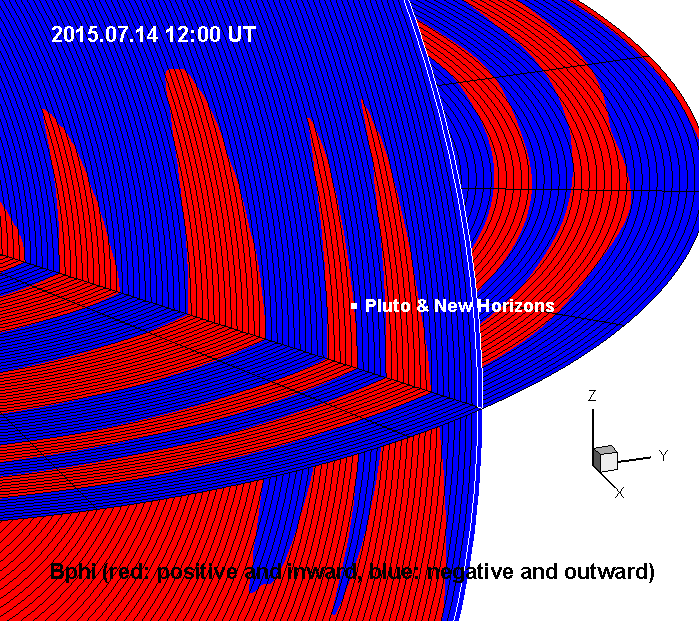
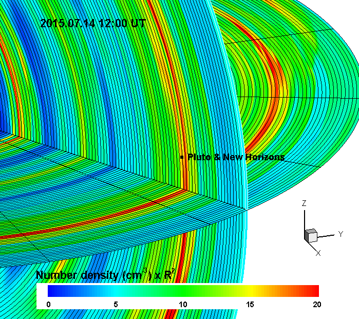
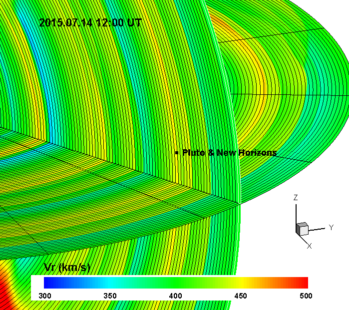
Preliminary Multi-Scale Fluid-Kinetic Simulation Suite (MS-FLUKSS) 3D MHD results from Tae Kim, Nikolai Pogorelov and Gary Zank
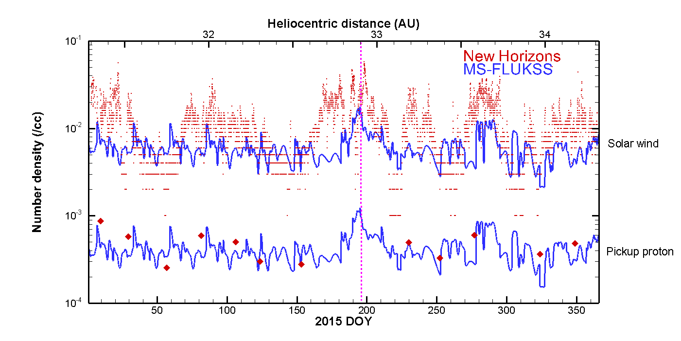
Line plots comparing the model predictions with the New Horizons measurements for solar wind and pick-up proton density, radial velocity, Bphi, temperature, Z2 (total turbulent energy density in turbulent magnetic and velocity fluctuations), correlation length lambda and Sigma_c for the year 2015. The model speed, density, and temperature are compared with New Horizons SWAP data (Elliott et al. 2016, ApJS, 223, 19; McComas et al. 2017, ApJS, 233, 8). Also shown are 3D plots of the density (scaled to 1 AU values by R^2) NxR2 (/cc), Vr (km/s), and Bphi sign (red: positive, blue: negative) at the time of the closest approach to Pluto. The 3D plots show the parameters on the equatorial plane and on a plane formed by the solar rotation axis (Z) and the Sun-Pluto line.

This model is a 3D, time-dependent, MHD-plasma/fluid-neutral code (e.g., Pogorelov et al. 2008, 2009; Kim et al. 2016) based on the Multi-scale Fluid-kinetic Simulation Suite (MS-FLUKSS; see Pogorelov et al. 2014 and references therein). This assumes a single plasma fluid coupled with a fluid description for neutral hydrogen through mass, momentum, and energy source terms.
References
- Kim, T. K., Pogorelov, N. V., Zank, G. P., Elliott, H. A., & McComas, D. J. (2016), ApJ, 832, 72
- Pogorelov, N., Borovikov, S., Heerikhuisen, J., et al. (2014), in Proc. 2014 Annual Conf. on Extreme Science and Engineering Discovery Environment (New York: ACM), 22
- Pogorelov,N.V., Borovikov,S.N., Zank,G.P., and Ogino,T.,(2009), ApJ, 696, 1478.
- Pogorelov,N.V., Zank,G.P., Borovikov,S.N., et al. (2008), in ASP Conf. Ser. 385, Numerical Modeling of Space Plasma Flows, ed. E.Pogorelov, E.Audit, and G.P.Zank (San Francisco, CA: ASP), 180.
1.5D MHD results from mSWiM - Kenneth Hansen (University of Michigan)
The plots below shows preliminary results from a simulation using the mSWiM code. mSWiM is a 1.5-D ideal MHD model implemented with the Versatile Advection Code (VAC), a general software package designed to solve a conservative system of hyperbolic partial differential equations with additional non-hyperbolic source terms [Tóth, 1996]. The model propagates the solar wind plasma radially outward from the Earth´s orbit at a selected helioecliptic longitude in the inertial frame of reference assuming spherical symmetry.
For a detailed description of the MHD equations, the numerical schemes used and a detailed validation of mSWiM, please refer to the paper by Zieger and Hansen [2008] or visit the model web site https://mswim.engin.umich.edu .
mSWiM has been used extensively by the outer planets community to study solar wind driven effects at Jupiter, Saturn and Uranus. Other applications of the model have included the inward propagation of the solar wind from the Earth to Mercury. See a complete bibliography below.
The simulation uses solar wind conditions measured at Earth as the inner boundary. We most commonly use hourly solar wind plasma and interplanetary magnetic field (IMF) data in the RTN coordinate system from the OMNIWeb database as input, but also use STEREO data as well as ACE data to make predictions in the outer solar system.
The first plot shows the model prediction for radial velocity and number density for the calendar year 2015, at both Pluto and the location of the New Horizons spacecraft.
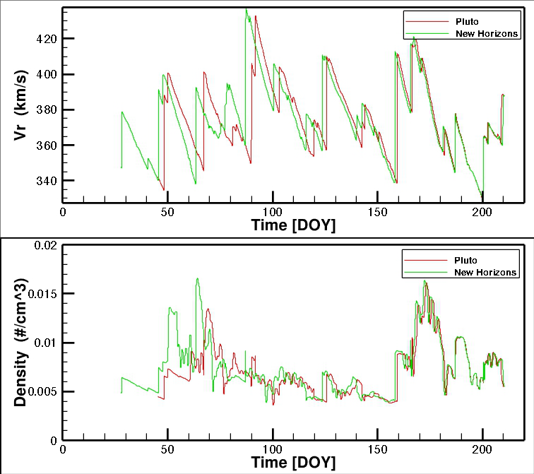
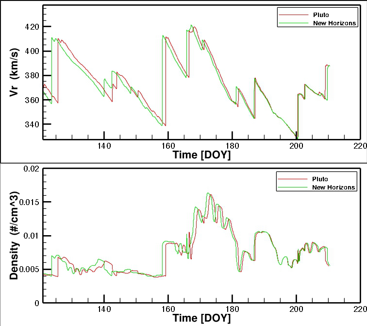
The second plot shows the same quantities as the first plot, but with the time window expanded to show just May to July, ie the time interval around the approach and the flyby at Pluto.
2D MHD results from SWMF-OH - Drs. Bertalan Zieger and Merav Opher(Boston University), Gabor Toth and Tamas Gombosi(University of Michigan)
The plots below shows preliminary results from a simulation using the Outer Heliosphere (OH) module of the Space Weather Modeling Framework(SWMF).
The code and the OH module is 3D MHD multi-fluid model. It evolves one ionized and up to four neutral H species as well as the magnetic field of the sun and interstellar magnetic field. For this particular calculation, the code modeled just the solar equatorial plane and two neutral species.
The ions and the magnetic field are driven by OMNI observations at 1AU. The usual trick is used to fill in the full circle by assuming that the solution does not change (much) for a Carrington rotation. The neutrals are driven by an inflow boundary in the negative X direction at 50AU distance. The neutrals are represented by 2 Maxwellian populations (fluids) and the densities, velocities and temperatures at the 50AU inflow boundary are based on previous 3D equilibrium model runs of the outer heliosphere. The model is run in a time accurate mode in the inertial HGI coordinate system. Spherical expansion effects are properly taken into account for the ions and the solar magnetic field. The neutrals, on the other hand, flow parallel with the equatorial plane. The ions and neutrals interact via the collision terms described in the papers by Merav Opher et al (see below).
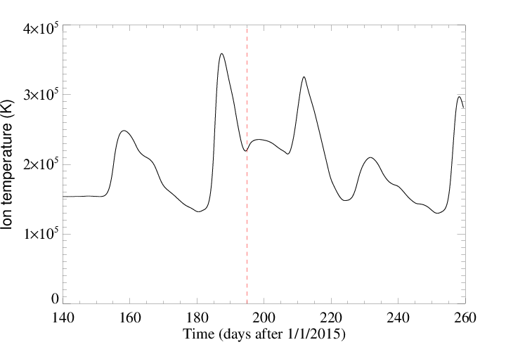
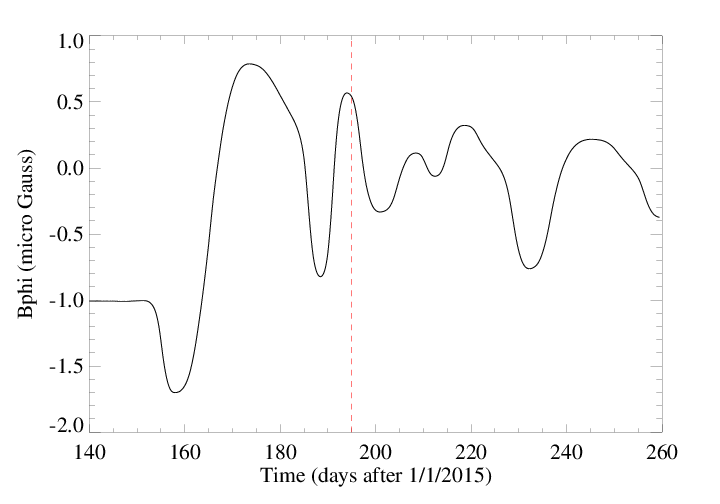
The first pair of plots shows the radial wind speed in the equatorial plane at the time of closest approach in the left frame, and the solar wind proton temperature in the right frame. The black plus sign is Pluto.


The next set of plots shows timelines of the solar wind number density, velocity, temperature and Phi component of magnetic field as a function of time at New Horizons between May 1, 2015 and August 9, 2015.
This 2D movie shows the evolution of the solar wind velocity in the solar equatorial plane from January 28 to September 16, 2015. This is in HGI coordinates. Pluto is located at approximately x=-29,y=-15 in this movie.
)
More information about this model can be found in the following papers:
- M. Opher, E. C. Stone, and P. C. Liewer, “Effects of a Local Interstellar Magnetic Field on Voyager 1 and 2 Observations”, The Astrophysical Journal, 640, L71 (2006).
- M. Opher, E. C. Stone, and P. C. Liewer, “Effects of a Local Interstellar Magnetic Field on Voyager 1 and 2 Observations”, The Astrophysical Journal, 640, L71 (2006).
- M. Opher, E. C. Stone, and T. I. Gombosi, “The Orientation of the Local Interstellar Magnetic Field”, Science, 316, 875 (2007).
- M. Opher, F. Alouani Bibi, G. Toth, J. D. Richardson, V.V. Izmodenov, and T. I. Gombosi, “A Strong highly-tilted Interstellar Magnetic Field near the Solar System”, Nature, 462, 1036 (2009).
- G. Toth, et al. (including M. Opher), “Adaptive Numerical Algorithms in Space Weather Modeling”, Journal of Computational Science, 231, 870 (2012).
- B. Zieger, M. Opher, N. A. Schwadron, D. J. McComas, and G. Toth, “A slow bow shock ahead of the heliosphere”, Geophysics Research Letters, 40, Issue 12, 2923 (2013).
- Opher, M., Drake, J. F., Zieger, B., Gombosi, T. I. Magnetized Jets Driven by the Sun: The Structure of the Heliosphere Revisited, Astrophysical Journal Letter, 800, L28 (2015).
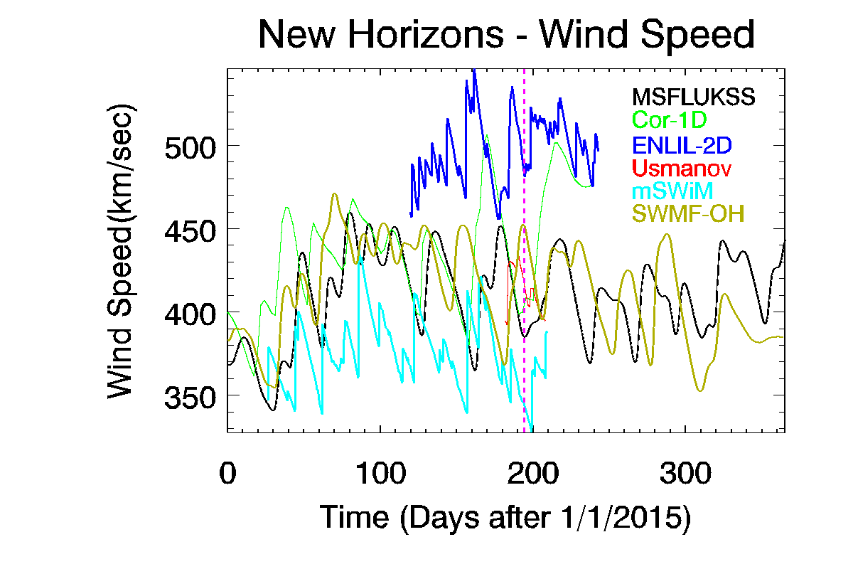
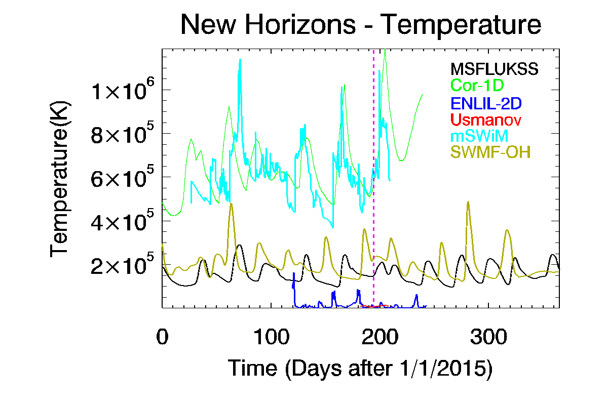
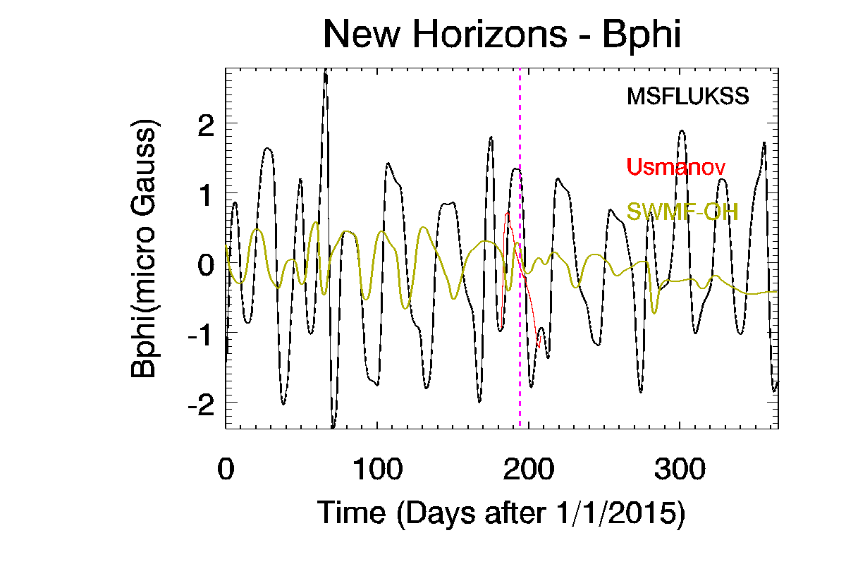
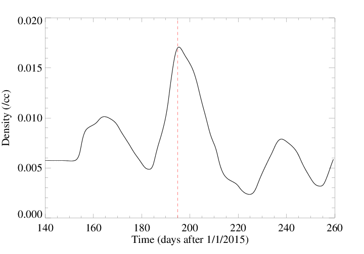
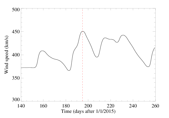
Ensemble Plots
These plots compare results from all the participating models. The vertical dashed magenta line indicates the time of the New Horizons fly-by of Pluto.