Kameleon Software Suite
What Kameleon can do for you!
Kameleon Design Goals
Primary goal: to facilitate scientific analysis of CCMC-supported models.
Kameleon Scope
Kameleon serves two primary functions:
- as a standard format for storing Space Weather Model output
- as a standard interface for model output

Quick Start Instructions
Quick Start Instructions
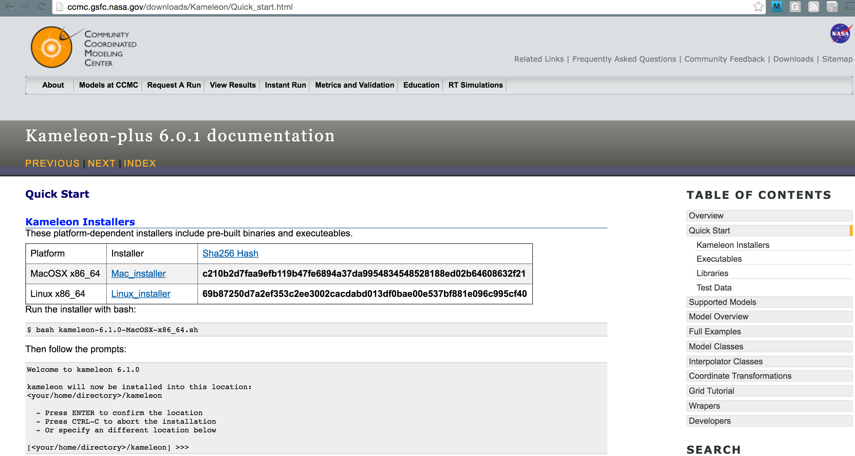
Kameleon Installers
These platform-dependent installers include all pre-built binaries, executeables, and prerequisits.
| Platform | Installer | Sha256 Hash |
|---|---|---|
| MacOSX >= 10.6 | Mac Installer | c210b2d7faa9efb119b47fe6894a37da9954834548528188ed02b64608632f21 |
| Linux x86_64 | Linux Installer | 69b87250d7a2ef353c2ee3002cacdabd013df0bae00e537bf881e096c995cf40 |
Running the installer
via bash:
bash kameleon-6.1.0-MacOSX-x86_64.sh
Then follow the prompts:
Welcome to kameleon 6.1.0

kameleon will now be installed into this location:
<your/home/directory>/kameleon

  - Press ENTER to confirm the location
  - Press CTRL-C to abort the installation
  - Or specify an different location below

[<your/home/directory>/kameleon] >>> my/path/to/install/kameleon
Running the installer
After chosing your install location preference, choose whether to prepend the kameleon install location to your system path:
Do you wish the installer to prepend the kameleon install location
to PATH in your /Users/apembrok/.bash_profile ? [yes|no]
[yes] >>> no
Since the kameleon installer includes its own version of python, saying yes would give Kameleon's python preference over your system pythons.
Installer Executables
When the installer finishes, the following executables will be placed in
my/path/to/install/kameleon/bin/ccmc/examples| subdirectory | executable | Description |
|---|---|---|
| c++ | kameleon_prog | opens and samples kameleon supported Model |
| time_interp | tests interpolation between time steps | |
| tracer_prog | tests the field line tracer on supported models | |
| integrator_prog | tests field line integrator on supported models | |
| coordinate_transformation_test | tests cxform's coordinate transformations | |
| lfm_test | tests the reader and interpolator for LFM | |
| enlil_test | tests the reader/interpolator for Enlil | |
| adapt3d_test | tests the reader/interpolator for Adapt3d | |
| open_ggcm_test | tests the reader/interpolator for open-GGCM | |
| mas_test | tests the reader/interpolator for MAS | |
| swmf_iono_test | tests the reader/interpolator for SWMF ionosphere model | |
| CDFReader | tests the reader CDF file reader |
| language | executable | Description |
|---|---|---|
| c | filereader_compat_test | tests c wrapper for filereader |
| kameleon_compat_test | tests c wrapper for kameleon | |
| time_interp_c | tests c wrapper for time interpolator | |
| tracer_c | tests c wrapper for tracer | |
| fortran | generalfilereader_compat_f | tests FORTRAN wrapper for general file reader |
| kameleon_compat_f | tests FORTRAN access to models through Kameleon | |
| timeinterp_compat_f | tests FORTRAN compatibility for time interpolator | |
| tracer_compat_f | tests FORTRAN compatibility for field line tracer | |
| time_series_test | saves time series of multiple variables to an output file |
| language | executable | Description |
|---|---|---|
| python | kameleon_test.py | tests python access to kameleon objects |
| tracer.py | tests python access to field line tracer | |
| ARMS_test.py | tests python access to ARMS reader (python plugin) | |
| grid.py | basic grid interpolation/cut plane visualization | |
| pyModel_test.py | test of embedded python readers/interpolators | |
| ionosphere_test.py | inspects ionosphere output and visualizes with plotly |
Installer Libraries
The installer includes the following platform-dependent libraries (names corresponding to a Mac build shown here). The example programs automatically link to these. The library paths will begin with
/path/to/kameleon/lib/ccmc
Headers are in
/path/to/kameleon/include/ccmc| library path | library name | Description |
|---|---|---|
| lib/ccmc/ | libccmc.dylib, libccmc_static.a | main ccmc library containing model readers, interpolators, and tools |
| lib/ccmc/ | libccmc_wrapper_c.dylib | c wrapper for ccmc library |
| lib/ccmc/ | libccmc_wrapper_fortran.dylib | fortran wrapper for ccmc library |
| lib/ccmc/ | pyKameleon.so | plugin module for python readers/interpolators |
| lib/python2.7/site-packages/ccmc | CCMC.py, _CCMC.so | python module |
Example: Interpolating within ENLIL
| Model name | model output | Runs on request run id |
|---|---|---|
| Enlil | Enlil output | Ailsa_Prise_101414_SH_1 |
| LFM | LFM output | |
| MAS | Mas output | |
| SWMF | SWMF output | Zheng |
| OpeGGCM | GGCM output | Alexa_Halford_062105_2 |
Download, untar and unzip any of the above test data, e.g.:
cd my/path/to/install/kameleon/bin/ccmc/c++
wget http://ccmc.gsfc.nasa.gov/downloads/sample_data/ENLIL.tar.bz2
tar -vxjf ENLIL.tar.bz2
Example: kameleon_prog
usage:
./kameleon_prog
kameleon <filename> variable c0 c1 c2
    Adapt3D, OpenGGCM, BATSRUS: x y z
    ENLIL, MAS: r theta(latitude) phi(longitude)
demo:
./kameleon_prog Ailsa_Prise_101414_SH_1.enlil.0001.cdf rho -30 0 0
r exists
loaded r
loaded lat
main: opened file: /Users/apembrok/Work/RoR_Sample_Data/ENLIL/Ailsa_Prise_101414_SH_1.enlil.0001.cdf with status: 0
main: kameleon file was opened successfully
starting interpolations
value: -1.09951e+12
deleting interpolator
Kameleon::close() calling model's close
This program assumes the user knows the model's coordinate system, but you may also work in your preferred coordinate system. See our Coordinate Transformations Tutorial for details.
Example: grid.py
Kameleon ships with a grid interpolation program:
usage: grid.py [-h] [-v] [-ginfo] [-db DEBUG] [-lvar] [-vinfo var]
           [-vars var1 [var2 ...]] [-pout]
           [-pfile /path/to/input/positions.txt] [-p px py pz]
           [-x xmin xmax] [-y ymin ymax] [-z zmin zmax] [-res nx [ny ...]]
           [-xint xint] [-yint yint] [-zint zint] [-order ordering]
           [-t TRANSFORM TRANSFORM TRANSFORM] [-vis] [-rows plot rows]
           [-cols plot columns] [-slice0 c0 index] [-slice1 c1 index]
           [-slice2 c2 index]
           [-pcoords <x-axis> <y-axis> <x-axis> <y-axis>]
           [-levels number contours] [-cvals var1_min [var1_max ...]]
           [-pgv] [-o path/to/output_file]
           [-f <flags><width><.precision><length>specifier] [-d ' ']
           [-ff fits [md ...]]
           full/path/to/input_file.cdf
Use python grid.py -h for full options.
Querying global attributes
!python grid.py -ginfo 3d__var_1_e20150315-000000-000.out.cdf
Global Attributes:
	README : Model Description:  BATS-R-US, the Block-Adaptive-Tree-Solarwind-Roe-Upwind-Scheme, was developed by the Computational Magnetohydrodynamics (MHD) Group at the University of Michigan,now Center for Space Environment Modeling (CSEM). It was designed using the Message Passing Interface (MPI) and the Fortran90 standard and executes on a massively parallel computer system.  The BATS-R-US code solves 3D MHD equations in finite volume form using numerical methods related to Roe's Approximate Riemann Solver. BATSRUS uses an adaptive grid composed of rectangular blocks arranged in varying degrees of spatial refinement levels. The magnetospheric MHD part is attached to an ionospheric potential solver that provides electric potentials and conductances in the ionosphere from magnetospheric field-aligned currents. Model Authors/Developers: Dr. Tamas Gombosi, University of Michigan,Center for Space Environment Modeling (CSEM) Model Input Parameters: Inputs to BATS-R_US are the solar wind plasma (density, velocity, V_x, V_y, V_z, temperature) and magnetic field (B_x, B_y, B_z) measurement, transformed into GSM coordinates and propagated from the solar wind monitoring satellite's position propagated to the sunward boundary of the simulation domain. The Earth's magnetic field is approximated by a dipole with updated axis orientation and co-rotating inner magnetospheric plasma or with a fixed orientation during the entire simulation run. The orientation angle is updated according to the time simulated or a fixed axis position can be specified independently from the time interval that is simulated. Model Outputs: Outputs include the magnetospheric plasma parameters (atomic mass unit density N, pressure P, velocity V_x, V_y, V_z, magnetic field B_x, B_y, B_z, electric currents, J_x, J_y, J_z) and ionospheric parameters (electric potential PHI, and Hall and Pedersen conductances Sigma_H, Sigma_P).
	model_name : batsrus
	model_type : Global Magnetosphere
	generation_date : 2016-01-11T00:00:00.000Z
	original_output_file_name : 3d__var_1_e20150315-000000-000.out
	generated_by : Zheng
	terms_of_usage : For tracking purposes for our government sponsors, we ask that you notify the CCMC whenever you use CCMC results in a scientific publications or presentations: ccmc@ccmc.gsfc.nasa.gov
	grid_system_count : 1
	grid_system_1_number_of_dimensions : 3
	grid_system_1_dimension_1_size : 15744
	grid_system_1_dimension_2_size : 15744
	grid_system_1_dimension_3_size : 15744
	grid_system_1 : [ x, y, z ]
	output_type : Global Magnetospheric
	standard_grid_target : GSM
	grid_1_type : GSM
	start_time : 2015-03-15T00:00:00.000Z
	end_time : 2015-03-20T02:00:00.000Z
	run_type : event
	kameleon_version : 5.4.0
	elapsed_time_in_seconds : 0.0
	number_of_dimensions : -3
	special_parameter_g : 1.66666996479
	special_parameter_c : 2997.89990234
	special_parameter_th : 0.101020999253
	special_parameter_P1 : 1.0
	special_parameter_P2 : 1.0
	special_parameter_P3 : 1.0
	special_parameter_R : 2.5
	special_parameter_NX : 8.0
	special_parameter_NY : 8.0
	special_parameter_NZ : 8.0
	x_dimension_size : 1007616
	y_dimension_size : 1
	z_dimension_size : 1
	current_iteration_step : 2500
	global_x_min : -224.0
	global_x_max : 32.0
	global_y_min : -128.0
	global_y_max : 128.0
	global_z_min : -128.0
	global_z_max : 128.0
	max_amr_level : 7.0
	number_of_cells : 1007616
	number_of_blocks : 1968
	smallest_cell_size : 0.25
	r_body : 2.5
	r_currents : 3
	dipole_time : N/A
	dipole_update : T
	dipole_tilt : 0.101020999253
	dipole_tilt_y : 0.0
Querying variable attributes
!python grid.py -vinfo rho 3d__var_1_e20150315-000000-000.out.cdf
rho [ amu/cm^3 ]
	valid_min : 0.0
	valid_max : 9.99999995904e+11
	units : amu/cm^3
	grid_system : grid_system_1
	mask : -1.09951162778e+12
	description : atomic mass density, limit may bee exceeded in dense atmosphere; solar corona 2e8
	is_vector_component : 0
	position_grid_system : grid_system_1
	data_grid_system : grid_system_1
	actual_min : 0.445019990206
	actual_max : 51.3815002441
Single point interpolation
The --variables options allows for multiple variables.
!python grid.py 3d__var_1_e20150315-000000-000.out.cdf --variables rho bx by bz -p -30 0 0
rho[amu/cm^3]       bx[nT]       by[nT]       bz[nT]
       0.499       13.245       -1.483       -0.929
Specifying a grid
A grid may be generated in cartesian (or spherical?) coordinates. Parameters for specifying the grid are as follows:
-res <ni> <nj> <nk>Grid resolution in each dimension-x <xmin> <xmax>.Inclusive range of x. If not specified, a constant value of x-intercept = 0 will be used.-xint <x-intercept>overriedes default x-intercept. Ignored if-xis set.-y <xmin> <xmax> -yint <y-intercept> -z <zmin> <zmax> -zint <z-intercept>same as above.-order 'F'for Fortran-style column major. Positions will be in row major by default.
Example - Planar output
This command computes variables on a 2 x 3 plane at x = -30 with fortran ordering:
!python grid.py 3d__var_1_e20150315-000000-000.out.cdf -xint -30 -y -10 10 -z -10 10 -d ' ' -f "12.3f" -order 'F' -res 1 3 4 -vars rho ux bx by bz
rho[amu/cm^3]     ux[km/s]       bx[nT]       by[nT]       bz[nT]
       1.169     -125.765      -15.363       -4.257       -3.898
       0.714     -134.060      -16.312       -1.708       -4.259
       0.959     -122.368      -15.662        0.949       -4.151
       0.812     -358.504       -8.094       -2.803       -1.962
       0.497     -475.728       -7.024       -1.801       -1.514
       0.768     -411.462       -5.257       -0.806       -1.407
       0.808     -136.027       16.051        1.502       -1.953
       0.651     -140.673       16.948       -1.415       -1.939
       1.402     -122.243       15.823       -3.802       -1.627
       0.896     -121.704       16.414        0.711       -2.244
       0.875     -124.435       17.080       -1.578       -2.329
       1.228     -124.613       16.135       -2.957       -1.634
Example - Volume output
This command computes variables on a 2 x 3 plane at x = -30 with fortran ordering. The result is stored in tmp/batsrus_output.txt.
Alternative formats include json and idl.
!python grid.py 3d__var_1_e20150315-000000-000.out.cdf -x -10 -50 -y -10 10 -z -10 10 -res 2 2 3 -vars rho ux bx by bz -f "12.3f" -v -o /tmp/batsrus_output.txt
Running grid interpolator.
loading 5 desired variables: ['rho', 'ux', 'bx', 'by', 'bz']
exclusing positions from output
requested output resolution: [2, 2, 3]
x-range: [-10.0, -50.0]
y-range: [-10.0, 10.0]
z-range: [-10.0, 10.0]
output resolution: (2, 2, 3)
writing ASCII to /tmp/batsrus_output.txt.txt
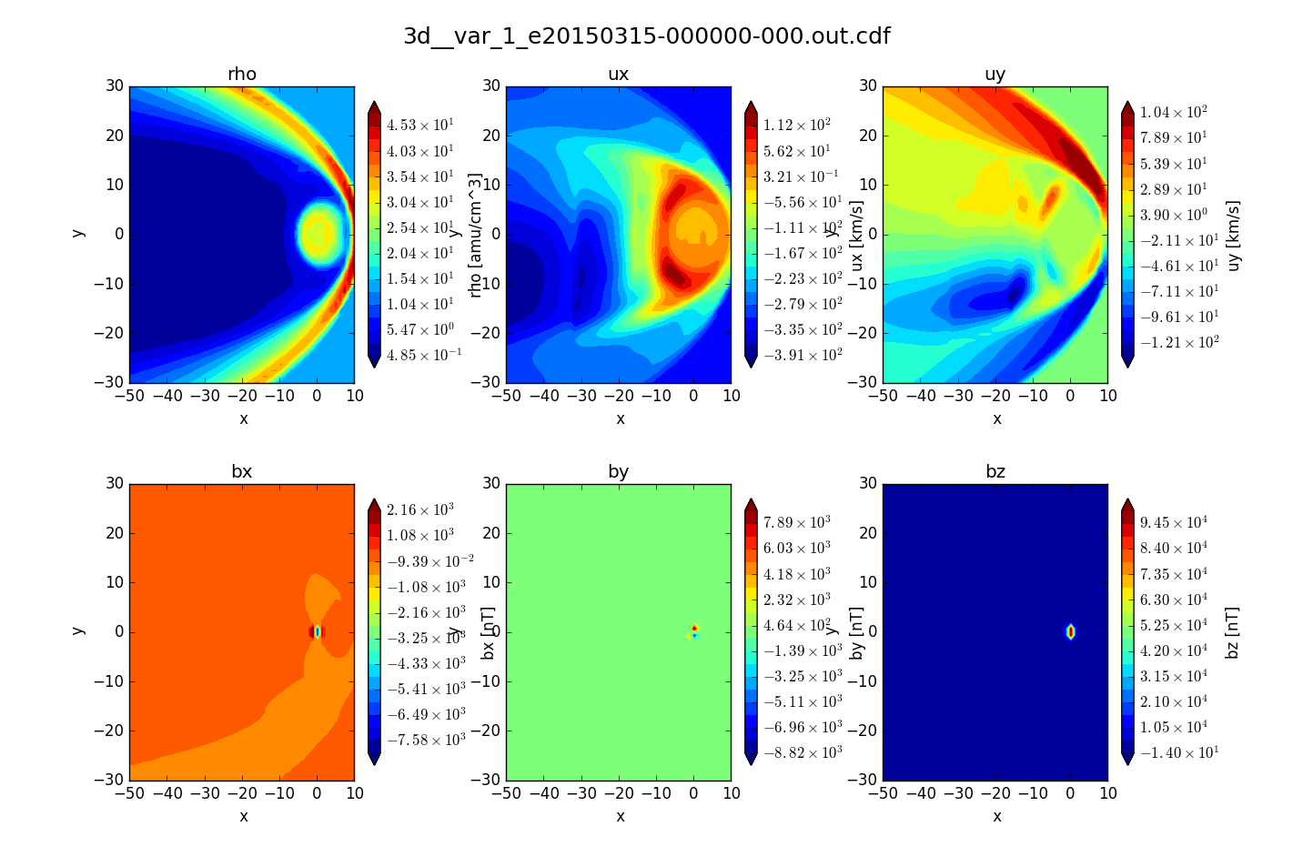
Visualization with matplotlib
Include the -vis option to generate matplotlib images of slice query.